Convolutional DCT

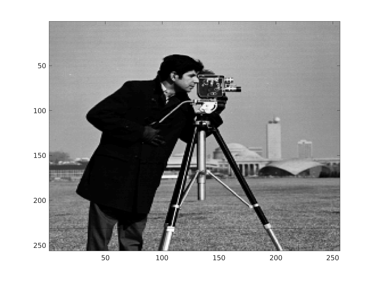
This example shows how an overlapped block dct transform can be calculated using n-dimensional correlations. First, let's load an image:

im = double(imread('cameraman.tif'));
figure; imagesc(im);
colormap gray;

conv_dct:image.png

For the calculation of the transform and its inverse, 3 operations are needed:

correlate all 2d DTC basis functions with the image
correlate all feature maps in the third dimension with 1x1xN filters in order to calculate the inverse transform
correlate the reconstructed image with a 3D filter performing reconstruction. This operation basically averages over all blocks containing a pixel in order to reconstruct that pixel.

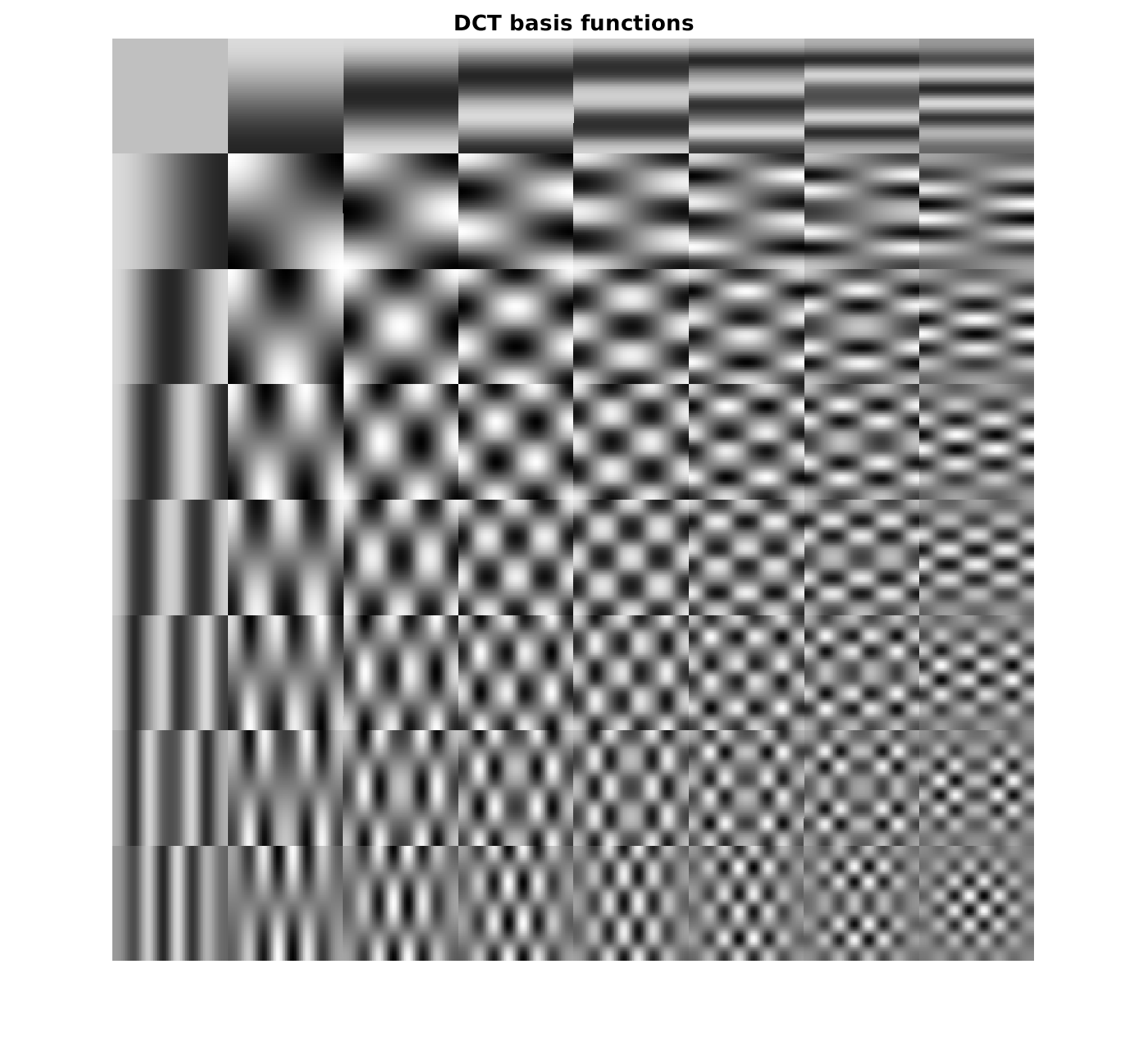
So let's define the DCT basis functions

% generate vectorized DCT transform matrix for 8x8 blocks
D_dct = kron(dctmtx(8),dctmtx(8))';

% reshape the DCT matrix and its inverse (transposed), store it as cell
% array. In the cell array, we have the block basis functions
D = reshape(D_dct,[8,8,64]);
Dt = reshape(D_dct',[8,8,64]);
DasCell = mat2cell(D,8,8,ones(64,1));
DtasCell = mat2cell(Dt,8,8,ones(64,1));

figure; montage(D,'DisplayRange',[]);
title('DCT basis functions');

conv_dct:dict.png

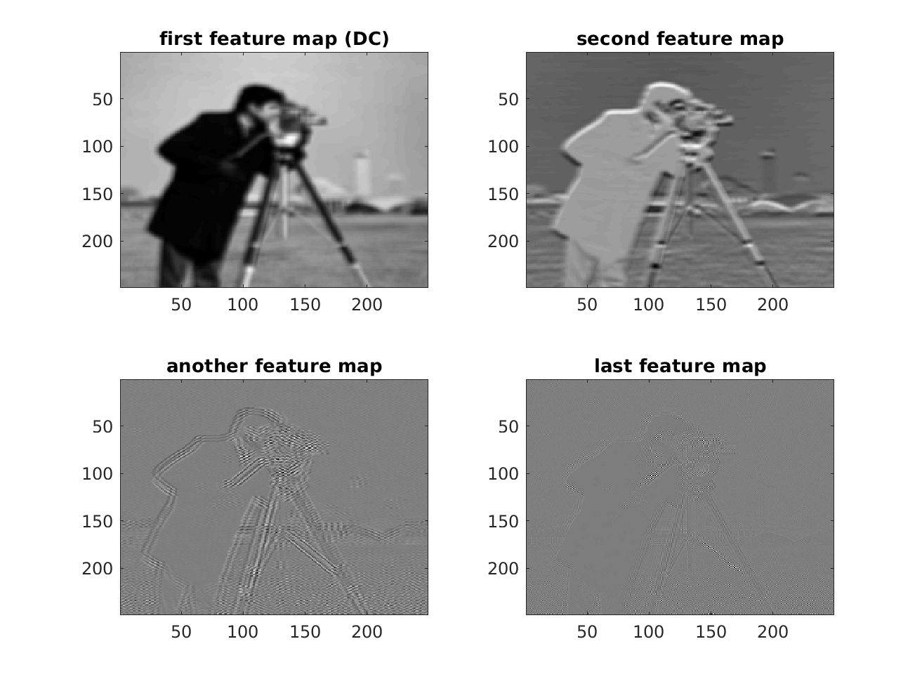
Implementation-wise, operations are performed as cellfuns, if a correlation with multiple filters should be calculated (referring to a layer in a CNN). So, let's calculate the feature maps:

% flip the basis functions since we want to calculate correlations instead
% of convolutions
DtasCell = cellfun(@(x) reshape(flipud(x(:)),size(x)), DtasCell,'un',0);

% calculate the DCT transform and store the coefficients in feature maps
featureMaps = cellfun(@(x) conv2(im,x,'valid'),DtasCell,'un',0);

figure; 
subplot(2,2,1);
imagesc(featureMaps{1}); colormap gray;
title('first feature map (DC)');

subplot(2,2,2);
imagesc(featureMaps{2});
colormap gray
title('second feature map');

subplot(2,2,3);
imagesc(featureMaps{30});
colormap gray
title('another feature map');

subplot(2,2,4);
imagesc(featureMaps{end});
colormap gray
title('last feature map');        

% store the feature maps as n-dimensional array so that it can be processed
% further by n-dimensional fitlers
featureMapsAsnDArray = cell2mat(featureMaps);

conv_dct:featuremaps.png

Now you are wondering, why one would calculate a dct like that, since the transform is highly redundant, when it is applied on overlapped blocks. However, there are scenarios where you do not have orthogonal transforms in image processing. In this case the procedure might be useful, as the content is analysed in the first correlation operation, and the feature maps can be further processed (thresholding, relu, sigmoid, whatever you want) and the image can be reconstructed. Thereby, the transformation can be learned, if handcrafted basis function do not fit the needs of the application. This is a very basic example of CNN-based image processing.

Moreover, you are wondering, how you can get a non-overlapped block transform. For this, you basically need to adjust the convolution stride to the block size of the transform. However, matlab does not offer the possibilty to adjust the convolution stride directly, but we can mimic this operation by downsampling after correlating. For sure, upsampling has to be performed during reconstruction in that case. This is often referred to as a deconvolutional layer in deep learning. However, this term is somewhat misleading as the basic operation still stays the same - correlation or convolution. I think the interpetation of a correlation operation with a fractional stride describes best, what is going on in a deconvolutional (or also called transposed convolutional) layer.

After this very short discussion, let's apply the inverse DCT to our featuremaps:

% generate the filters for calculation of the inverse DCT
invDct = mat2cell(D_dct,64,ones(64,1));
invDct = cellfun(@(x) reshape(x,1,1,numel(x)),invDct,'un',0);

% flip the filters as we want to calculate the correlation and not
% convolution
invDct = cellfun(@(x) reshape(flipud(x(:)),size(x)), invDct,'un',0);

% calculate the reconstruction. Note that we have reconstructions for every
% position where our filter was operated.
recon = cellfun(@(x) convn(featureMapsAsnDArray,x,'valid'),invDct,'un',0);

% store the reconstruction maps as n-dimensional array so that it can be processed
% further by n-dimensional fitlers
reconAsnDArray = cell2mat(reshape(recon,1,1,numel(recon)));

conv_dct:inverse.png

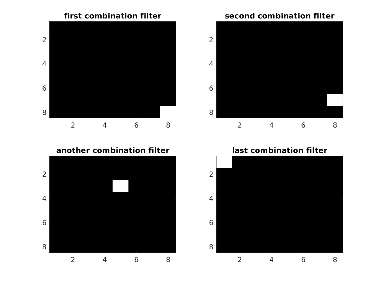
Now, we have the reconstruction for every featuremap and we need to combine them back to an image, in order to perform step 3 of the list from the start. Since the feature maps store the orginal image at shifted positions, we can combine them by shifting and averaging. Let's design a filter for that:

% desing a combination filter. Note that it is only averaging in
% overlapping areas here
combineFilter = reshape(rot90(eye(64)),8,8,64)/64;
figure; 
subplot(2,2,1);
imagesc(combineFilter(:,:,1));
colormap gray
title('first combination filter');

subplot(2,2,2);
imagesc(combineFilter(:,:,2));
colormap gray
title('second combination filter');

subplot(2,2,3);
imagesc(combineFilter(:,:,30));
colormap gray
title('another combination filter');

subplot(2,2,4);
imagesc(combineFilter(:,:,end));
colormap gray
title('last combination filter');

conv_dct:combinationfilter.png

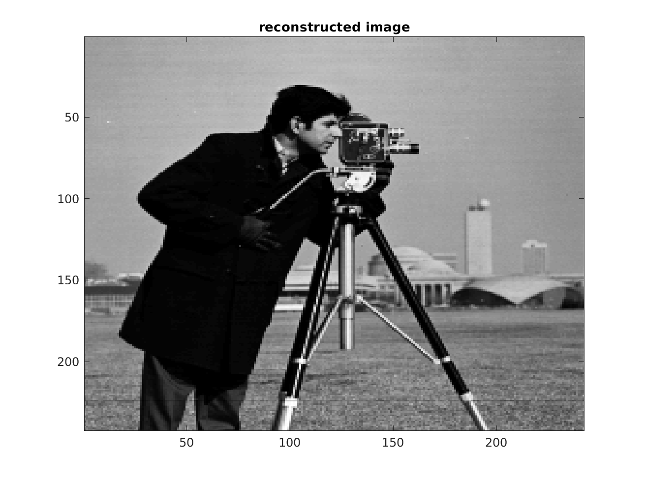
Now we get the reconstructed image by filtering the featuremaps with the combination filter:

% calculate the reconstructed image. Note that it is smaller than the
% original image due to boundary effects of the correlation operations.
reconImage = convn(reconAsnDArray,combineFilter,'valid');

figure; imagesc(reconImage);
colormap gray
title('reconstructed image');

conv_dct:reconstruction.png